

Start working more efficiently with Excel VLOOKUP. If you’ve ever found yourself struggling to search and retrieve specific data within your Excel spreadsheets, then you’re in the right place. Here, we will provide you with an Excel VLOOKUP tutorial, uncovering the key techniques to streamline your data analysis.
Learn the fundamental concepts of VLOOKUP, the common challenges and solutions. Soon, you will be armed with the knowledge and confidence to use Excel VLOOKUP in your own projects.
Why Use the Excel VLOOKUP Function?
The Excel LOOKUP function searches for a specific value in a column so it can return a value from another column in the same row. Basically, it can save you hours of manually copying and pasting data from one column range to another. Other advantages include:
- Speeds up data analysis
- Improves accuracy
- Boosts productivity
What is Excel VLOOKUP?
VLOOKUP stands for ‘Vertical Lookup’ as it can retrieve data from a vertical orientation. VLOOKUP is a function used to search for data in a specific table, range, or row and retrieves a value in the same row from another column. Read on for a detailed step-by-step example.
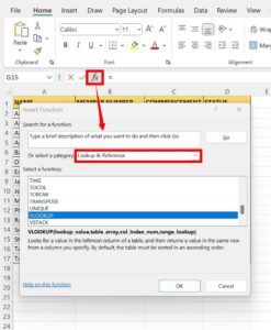
To use Excel VLOOKUP function, you can either type the formula directly into the cell, or use the ‘Insert Function’ button and search for VLOOKUP.
Syntax of VLOOKUP
The syntax of Excel VLOOKUP function includes:
- lookup_value: this is the value to search for in the first column of the table.
- table_array: this is the table of data in which to perform the lookup.
- col_index_num: this specifies which column number in the table_array that the matching data should be returned.
- range_lookup: this can be either TRUE or FALSE. If TRUE or omitted, it assumes the first column is sorted either in ascending order (smallest to largest) or descending order. If FALSE, it requires an exact match.
Excel VLOOKUP example below.
How Excel VLOOKUP Works
The Excel VLOOKUP function searches for a specific value (lookup_value) in the first column of a table (table_array). Once it finds a match, it retrieves the value in the same row based on the specified column number. In simple terms, VLOOKUP helps you quickly find and pull relevant data from a large dataset based on specific criteria.
Excel VLOOKUP tutorial:
Excel VLOOKUP example in detail:
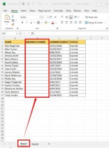
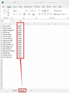
On sheet 1, we have a table listing our customer membership information. On sheet 2 is some raw data extracted from the customer database system. In this example, we want to pull all the membership numbers across from sheet 2 (column B) and insert them into the ‘Member Number’ column in our table in sheet 1 (column B).
1. Click on sheet 1 → click on the top cell of the column you want to pull information into (column B).
2. Add in the VLOOKUP formula: =VLOOKUP(
3. Select the data in the ‘Names’ column → add a comma in the formula: =VLOOKUP(A2:A17,
4. Now add the range where you want Excel to look for the data. In this example, it’s the membership numbers on sheet 2 (column B). Click on sheet2 tab, this will automatically add into the formula so it will look like this: =VLOOKUP(A2:A17, ‘Sheet2’!
5. Select both the names and member number columns. The A1:B16 is the range of the names and member number cells combined. Add another comma in the formula. It will now look like this: =VLOOKUP(A2:A17, ‘Sheet2’!A1:B16
6. Out of that data range, we must tell Excel that it’s the membership data in the second column (B) that we want in our table in sheet 1. To do this, type 2 in the formula followed by a comma. It will look like this: =VLOOKUP(A2:A17, ‘Sheet2’!A1:B16,2,
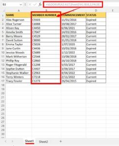
7. We want the exact information so type ‘FALSE’ in the formula → complete the formula with close parentheses. It will look like this: =VLOOKUP(A2:A17,Sheet2!A1:B16,2,FALSE)
8. Press enter → the member numbers from sheet 2 will now populate in column B in the table in sheet 1.
Note: if you want to bring across information from multiple columns, you can use XLOOKUP.
Formula breakdown
Earlier, we outlined the syntax of VLOOKUP. To make it easier to understand, this is how it appears in the formula =VLOOKUP(A2:A17,Sheet2!A1:B16,2,FALSE)
- =VLOOKUP() is the function command
- A2:A17 is the lookup_value
- Sheet2! Is the table_array
- A1:B16 Is the table_array
- 2 is the col_index_num
- FALSE is the range_lookup
Benefits of Excel VLOOKUP
When working with large datasets in Excel, the VLOOKUP function offers significant advantages that increases productivity and accuracy.
Handling Large Datasets
VLOOKUP handles large datasets effectively, so you can get specific information from extensive tables or databases. By automating the process of searching for/matching data, VLOOKUP eliminates the need for manual work, saving you valuable time. This feature streamlines data manipulation tasks and allows you to work more easily with complex datasets.
Reducing Errors
One of the best benefits of VLOOKUP is its ability to reduce errors in data retrieval and matching. Less manual handling of large data means less chance of human error. This makes it more reliable when making decisions based on the retrieved information.
Common Errors & Troubleshooting
Excel VLOOKUP is great for finding and extracting specific data from large datasets. However, it is possible to encounter errors or inaccuracies if not using it right. Understanding how to manage these issues is crucial to ensure the function works properly.
Handling #N/A Errors
One of the most common errors when using the Excel VLOOKUP function is the #N/A error. This occurs when the function can’t find the specified value in the lookup range. To troubleshoot this issue:
- Check the lookup value exists in the lookup range.
- Double check for any leading or trailing spaces.
- Check for any formatting differences.
- If the lookup value is numerical, confirm that the data types align with the lookup range.
Dealing with Inaccurate Results
Inaccurate results from VLOOKUP may be due to mismatched data types, unsorted lookup arrays, or incomplete data. To troubleshoot this issue:
- Ensure the lookup range is sorted in ascending order.
- Consider using the exact match parameter (FALSE) to avoid approximate matches.
- Verify the data types of the lookup values and lookup range to fix any discrepancies.
For additional information on Excel VLOOKUP troubleshooting, refer to Microsoft’s official troubleshooting guide.

Advanced Excel VLOOKUP Techniques
When it comes to mastering VLOOKUP, understanding some advanced techniques can take your data analysis to the next level.
Nested VLOOKUP
Nested VLOOKUP involves using an Excel VLOOKUP function within another VLOOKUP function to perform more complex data retrieval. This way, you can retrieve data based on multiple criteria and create relationships between the datasets.
E.g., use nested VLOOKUP to extract specific details from a master dataset that meets a set of conditions, which will provide a more refined data analysis.
Learn more about Nested VLOOKUP here.
Using Wildcard Characters
Wildcard characters, such as asterisks (*) and question marks (?), can be used within VLOOKUP to do partial matches and lookups. This is useful when dealing with unstructured datasets as it enables you to do more adaptable searches within the spreadsheets.
Handling Multiple Criteria Searches
Performing Excel VLOOKUP with multiple criteria allows for more intricate data analysis. By combining VLOOKUP with functions like IF, INDEX, and MATCH, you can create formulas that cater to specific conditions and criteria within your dataset. You can conduct more detailed searches, uncovering valuable insights into your data that may have been overlooked with a traditional VLOOKUP.
Start Using VLOOKUP and Boost Your Productivity
Mastering the VLOOKUP function is a game-changer for anyone working with data. To use this tool effectively, its important to understand the key components:
- Lookup value
- Table array
- Column index number
- Range lookup
By using Excel VLOOKUP you can streamline your data analysis and decision-making process and reduce time and errors. So, dive into this Excel function and unlock its full potential for your data tasks.