

After spending hours preparing a complex spreadsheet, the last thing you want is your formulas or layout tampered with. Accidents can happen, particularly when there are many fingers in the pie. Stay confident by learning how to protect cells in Excel:
- Lock cells
- Allow edit ranges
- Set up passwords
- Protect entire workbooks
How to Protect Cells in Excel
Lock Cells
1. Select the entire worksheet.
2. Home tab → Format Cells (via 1. font group, 2. alignment group or 3. Format drop-down list).

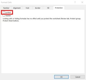
3. Go to Protection tab → untick ‘Locked’ → Ok.
4. Select the cells you want to lock.
5. Go back to Format Cells/Protection tab and tick ‘Locked.’
6. Go to Review tab → Protect Sheet.
7. You’re given a variety of restriction options (or you can stick with pre-selected 2).
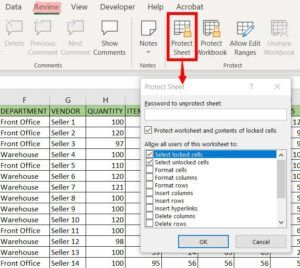
8. There is an option to create a password → Create a password and confirm.
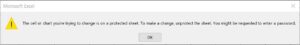
9. If anyone tries to alter the locked cells, they will be prompted with the message below. The other cells will still be accessible to edit.
To remove: go to Review tab → Unprotect Sheet.
Password options: if you don’t want a password, just leave it blank and press Ok. This means anyone can edit the cells by pressing ‘Unprotect Sheet.’
Protect Cells in Excel – Allow Edit Ranges
This allows a user to unlock certain cells on a protected worksheet. Rather than unprotecting the entire worksheet, the user can alter specific cells using a password.
1. Firstly, make sure your worksheet is currently unprotected (check via the ‘Unprotect Sheet’ button).
2. Select the range of cells you want to allow for editing.
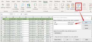
3. Go to Review tab → Allow Edit Ranges.
4. Your selected range should appear in the white box. Otherwise, press ‘New’, click on the ‘Refers to Cells’ box, and select your cells on the worksheet. The fixed formula should appear in this box.
5. You can create a password, or leave it blank to allow anyone to edit this range.
6. You can give some users permission to edit without a password by clicking the ‘Permissions’ button and adding their username (optional).
7. To add more ranges, repeat steps 4 and 5.
8. Click the ‘Protect sheet’ button → Ok.
Tip: you can also alter passwords in this box via the ‘Modify’ button.
Protect Entire Workbook
To protect the workbook structure:
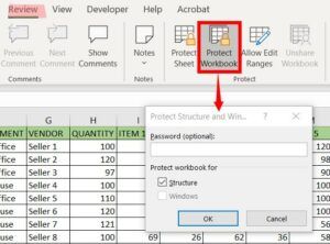
1. Go to Review tab → Protect Workbook.
2. You’re given the option to set a password, leave it blank if you don’t want to → Ok.
3. If you right-click on the worksheet tab, the options to modify (insert, delete, rename) are now inaccessible.
>>Click here to learn more about Excel tabs<<
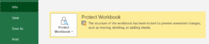
You can also confirm the protection status in the Review tab (‘Protect Workbook’ is highlighted). Or in File/Info (‘Protect Workbook’ is highlighted).
Password Protect Entire Workbook
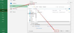
1. File → Save As.
2. Type in a file name.
3. Click on ‘More Options’ → Tools → General Options.
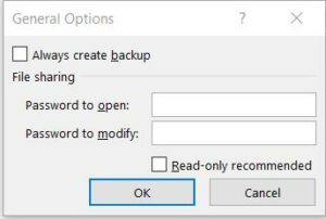
4. Create a file-sharing password and confirm. There’s also the option to recommend ‘Read Only’ → Save.
5. Users will be prompted for the password every time the file is opened. If you select ‘Read Only’ option, it will encourage users to open in that mode unless they need to make changes.
Having issues with formulas? Check out this helpful article: 10 tips for troubleshooting Excel formulas and functions
Protect Your Work
It’s worth it to take a few minutes to learn these functions. Protecting your spreadsheets can save you potential frustration and hours of rework from accidental edits.

Hi CJ, thanks for this post. I already knew how to protect a workbook but I didn’t know it was possible for individual cells and worksheets. I like the extra layer of security so I’ll be using this.
Hi TamikaG, I’m glad you found this helpful. Let me know if I can help with anything else 🙂