

Ever pull your hair out dealing with spreadsheets full of duplicate data? Trying to manually find duplicates in Excel can feel impossible at times. Not only is it too time-consuming, but it’s also tedious and easy to miss something. Luckily Excel has a function that does this task for you, fast and accurately. In this article you will learn:
- How to find duplicates in Excel
- How to highlight duplicates after the first instance
- How to filter and sort duplicates
- How to highlight unique values
- How to remove duplicates
Duplicates in Excel
Having duplicates in your spreadsheets is a common occurrence, especially when extracting raw data. You can use Excel’s conditional formatting to help you identify and filter this. By familiarising yourself with this tool, you’ll save time.
(Video breakdown: Find Duplicates 0.13, Duplicates After First Instance 0.40, Unique Values 1.13, Sort 1.34, Remove 2.00).
How to Find Duplicates in Excel
1. Select the range of cells you want to search.
2. Styles group → Conditional Formatting.
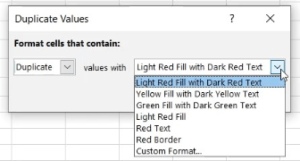
3. Highlight Cell Rules → Duplicate Values

4. Select a formatting style/colour → Ok.
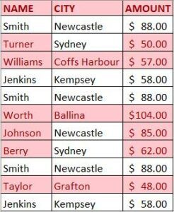
5. Excel will highlight all the cells that are duplicated (including the first instance).

Highlight Duplicates After the First Instance
Sometimes you might want to keep the first instance blank and highlight any duplicates after that. To do this, you need to create a formula in conditional formatting:
=COUNTIF (first cell of range fixed: first cell non-fixed, first cell non-fixed) greater than 1.
For example, my table begins in cell A1. So the formula will look like this: =COUNTIF($A$1:A1, A1)>1
- Select the range of cells you want to check.
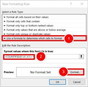
- Styles group → Conditional Formatting → New Rule.
- Select ‘Use a formula to determine which cells to format.’
- Type in the formula =COUNTIF($A$1:A1,A1)>1
- Go to Format → Fill → choose your colours and font → Ok.
- It will leave the first instance blank but highlight other duplicates.
Keyboard shortcut: Alt+O then D for conditional formatting manager.
>> Don’t know much about formulas? Learn the fundamentals of basic Excel formulas <<
How to Find Unique Values
You can also highlight the unique cells rather than the duplicates.
1. Select the range of cells you want to search.
2. Styles group → Conditional Formatting.
3. Highlight Cell Rules → Duplicate Values.
4. From the drop-down list, change to ‘Unique.’
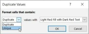
5. Select a formatting style/colour and click Ok.
6. The cells that aren’t duplicates will be highlighted.
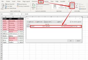
How to Sort Duplicated Cells
You may want to sort your highlighted cells. E.g. shift them all to the top and delete them in bulk.
- Select your cells.
- Go to Data tab → Sort.
- Select column, cell colour and order (on top).
- All highlighted duplicates will be moved to the top of the spreadsheet.
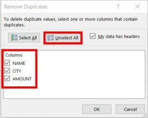
How to Remove Duplicates in Excel
- Click on a sell within the range you want to search.
- Go to the Data tab → Data Tools → Remove Duplicates.
- In the pop-up box, keep all boxes are ticked and press OK.

You can narrow this down further to specific columns. To do this, untick the columns you don’t need in the pop-up box.
E.g. if you want to remove people from the same town, untick all except the ‘City’ column. Excel will keep the first entry for that city and remove the rest.
Looking for More?
These articles cover more advanced training with duplicates:
How to highlight duplicate cells and rows in Excel
How to use macro examples to delete duplicate items in a list in Excel