
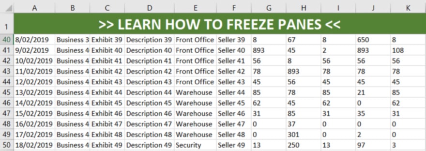
With large amounts of data, it’s difficult to compare rows from the bottom of the spreadsheet with the top (or even the middle).
Save yourself the hassle of scrolling and trying to remember details. Learn how to freeze the top row in Excel instead. Using this software, you can:
- freeze top row or first column
- freeze selection
- split worksheet to view horizontally or vertically
- split worksheet into four sections
- compare multiple workbooks.
Comparing data is easier than ever! See below for details.
How to Freeze the Top Row in Excel
- Click on a cell in the top row.
- Go to View tab → Freeze Panes → Freeze Top Row.
- The top row will now remain in view as you scroll down your document.

How to Freeze Selection
You can do the same for a selection of rows:
Go to View tab → Freeze Panes drop-down list → Freeze Panes.
This will keep the current selection frozen while you scroll through the remainder of the worksheet.
Keyboard Shortcut: alt+W then F, use the arrow buttons to scroll through the menu.
See the above video for a demonstration.
How to Freeze the First Columns in Excel
- Go to View tab → Freeze Panes → Freeze First Column.
- The first column will remain visible as you scroll across your document.
To freeze a selection of columns, you can use the ‘Freeze Panes’ option as above.
Keyboard Shortcut: Alt+W then F, use the arrow buttons to scroll down the menu.
See the above video for a demonstration.
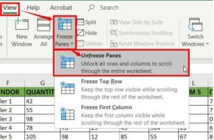
How to Unfreeze Rows and Columns
When you have a frozen pane, the ‘Freeze Panes’ function changes to ‘Unfreeze Panes.’
Go to ‘View’ tab → Unfreeze Panes.
Keyboard Shortcut: Alt+W then F, use the arrow buttons to scroll down the menu.
How to Split Window
You can’t freeze panes in the middle of your spreadsheet. But you can split your worksheet into sections. This enables you to scroll through some sections without affecting other areas of your worksheet.
- Click on a cell where you’d like the worksheet to be split.
- Go to View tab → Split.
- Grey lines will show the sections the worksheet has been split into. You can drag these lines to alter your sections.
Split horizontally: in column A, click on a cell where you want to split.
Split Vertically: in row 1, click on a cell where you want to split.
Split into 4 sections: click on a cell of your preference in the middle of the worksheet.
To return to normal, go back to the View tab and press ‘Split’ again. Or you can double-click on the section lines to make them disappear.

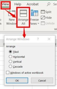
Comparing Multiple Workbooks
If you have multiple workbooks, you can compare them side-by-side too:
- Go to the ‘View’ tab → Arrange All.
- Choose whether you want to view them vertically, horizontally, etc.

Make the Most of it
These simple features are yet another great time-saving tool, making your job easier.
Know any other great hacks? Share your thoughts in the comments below!
More Spreadsheet Tips:
How to Create a Drop-down List, Autofill, and Flash Fill
How to Sort Tabs in Excel – Move, Colour Code & More