HOW TO CREATE EXCEL DROP-DOWN LIST, AUTOFILL & FLASH FILL

Learn to create an Excel drop-down list, use autofill, and flash fill functions to save you a ton of time. Excel can identify patterns, automatically display consecutive data, set up message alerts, and more. With these tools, you no longer need to type the same data over and over!

What are These Functions?

• Drop-down lists – just click on an arrow in the cell to choose your data from a list.
• AutoFill – create entire columns or rows of data based on the value of the first cell.
• Flash Fill – Excel can fill entire columns based on patterns of other columns.

Read on to learn more and discover how easy it is to use them.

How to Create an Excel Drop-down List

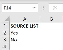
Create a list in Excel. For example, it could be a list of grocery items. Or simply ‘Yes’ and ‘No’.

1. On your existing worksheet, click on the cell/s where you want a drop-down list.

2. Go to Data → Data Validation → Settings tab.

3. In the ‘Allow’ drop-down menu, select ‘List.’

 

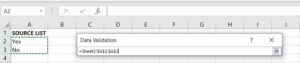
4. Click on the ‘Source’ field, then go to the list you created and select it.

5. Click on the small arrow to expand the Data Validation box again (bottom right corner of the floating field).

6. Press Ok.

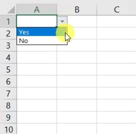
7. An arrow symbol will appear beside your cell to indicate there’s now a drop-down list.

8. Click on the arrow to pick from the list, which will appear in your cell.

Tip: If you have a long list, you can scroll with your arrow keys, or press alt+up/down arrow, or type the first few letters of the word.

How to Extend an Excel Drop-down List

There are a couple of ways to do this.

Copy & Paste

Simply copy the cell with the drop-down list and paste it to another cell.

Data Validation

1. Select the cell with the drop-down list and the cells beneath it that you want to include.

2. Go to Data Validation → You will get this message:

3. Click ‘Yes’ to open the Data Validation box (as shown above) → Ok.

4. The drop-down list will now appear on every cell you highlighted.

How to Update Data Validation List

To include more words in your drop-down list, go to your source list to add them. (E.g. in this case, add the word ‘Maybe’). If you have a long list of words, it’s best to sort them alphabetically.

Adding to this list won’t automatically update your drop-down list. You then need to:

1. Select the cell with an existing drop-down list.
2. Data Validation → Settings tab → click on the ‘Source’ field.
3. Select your updated source list (as shown previously) → Ok.

Alerts and Messages

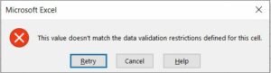
If you type a word that doesn’t exist in the drop-down list, you will get this alert:

To add the word to your list, follow the steps above.

However, you can also control error alerts to suit you. To do this:

1. Data Validation → Error Alert.
2. Untick the box ‘Show error alert after invalid data is entered.’

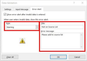
Or change the alert to a warning:

1. Data Validation → Error Alert.

2. In the ‘Style’ drop-down menu, change to ‘Warning.’

3. Add a title and error message (e.g. ‘Please add to source list’) → Ok.

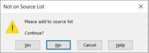
4. Now you can type a word that doesn’t exist, but you’ll first get this warning:

Or you can change the alert to information:

1. Data Validation → Error Alert.
2. In the ‘Style’ drop-down menu, change to ‘Information.’
3. Use the same title, description from the warning above.
4. Now you can type a word that doesn’t exist, but you’ll first get this message:

You can also input a message on the cell itself:

1. Data Validation → Error Alert.
2. Tick the box ‘Show error alert after invalid data is entered.’
3. Go to the ‘Input Message’ tab.
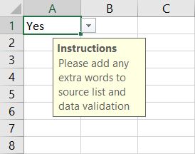
4. Enter a title and message → Ok.
5. Now, when someone clicks on the cell, they will see instructions.

How to Remove a Drop-down List

There are two ways you can do this:

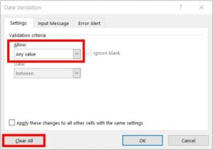
1. Data Validation → click on the ‘Clear All’ button → Ok.

Note: This will also clear any error messages and input alerts.

OR

2. Data Validation → in the ‘Allow’ drop-down menu, select ‘Any Value’ → Ok.

Note: this will not clear any alerts or input messages.

How to Use Flash Fill and AutoFill

Flash Fill

Excel picks up on any patterns of the data you’re filling in. This can be handy for filling columns with certain data instead of manually typing.

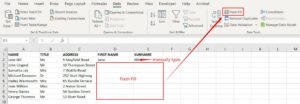
One good example is having customer information you want to separate for envelope labels.

1. Enter your data in the first row so Excel can establish a pattern.

E.g. Type data in column D (First Name) and column E (Surname) using the information in column A (Name).

2. Click on the next empty cell beneath.
3. On the Home tab go to Fill → Flash Fill (or Data tab → Flash Fill).
4. Excel will auto-populate the remaining cells, going off the pattern of information in the columns above.

Keyboard shortcut: ctrl+E

Autofill

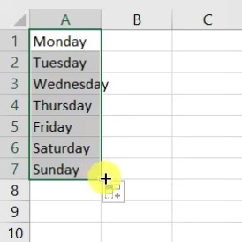
Instead of manually typing a lot of sequential data, you can use the Autofill function. Excel will calculate the proceeding cell data based on the value in the first cell.

1. Click on a cell and you’ll see a small green square in the bottom right corner.
2. Drag this icon down the column, or across the row.
3. The other cells will auto-populate with proceeding data (e.g. days of the week).
4. If you want the cells to copy the same (e.g. Monday, Monday, Monday) then hold the ctrl key as you drag the green square down or across.

Discover More

Follow more articles for helpful tips, such as how to freeze and split window, or colour and sort tabs.