

Do you realise you’re probably not using the Excel software to it’s full potential? Many users stick to the basics, not realising there are more functions of Excel that offer a wealth of benefits to improve productivity.
Join us as we uncover some of the hidden gems and explore how you can take your Excel skills to the next level. Incorporating these lesser-known functions are guaranteed to make a big difference in your data manipulation and analysis.
Text and Data Functions of Excel
In this section, we’ll dive into the practical applications of the TEXTJOIN function, the advantages of the CONCAT function over CONCATENATE, and the time-saving benefits of the FLASHFILL feature.
TEXTJOIN Function
The TEXTJOIN function in Excel lets you easily combine text from multiple cells into one cell, using a delimiter like a comma or space to separate the values.
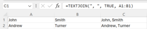
Example: You have a dataset with first names and last names in separate columns and need to combine them into a single column. The TEXTJOIN function allows you to easily do this, providing a seamless method for merging text values from different cells.
=TEXTJOIN(“, “, TRUE, A1:B1)
Here, “,” is the delimiter, ‘TRUE’ is used to ignore any empty cells, and A1:B1 is the range of cells containing the names.
CONCAT Function
The CONCAT function in Excel is an approved approach to the CONCATENATE function. It can handle ranges and arrays, making it easier to combine data from multiple cells or a specific range.
Example: You might use the CONCAT function when you need to create a single address line from separate cells containing different parts of the address. For example, if you have the house number in cell A1, the street name in B1, and the city in C1, you could use CONCAT to combine them into one cell.
Here’s how you could do it:
=CONCAT(A1, ” “, B1, “, “, C1)
This formula would take the values from cells A1, B1, and C1 and combine them into a single string with spaces and a comma, resulting in something like “123 Main Street, Sydney”.
FLASHFILL Feature
One of the powerful functions of Excel is FLASHFILL. This function performs automatic data filling based on patterns identified in the existing dataset. This capability can significantly improve your productivity by saving time and effort, especially when you’re dealing with repetitive data.
Example: If you have a list of names and need to extract the first names into a separate column based on a consistent pattern, the FLASHFILL feature can intelligently identify the pattern and automatically populate the new column. This can streamline your whole data organisation process.
Logical Functions of Excel
Understanding logical functions can be a game-changer to streamline your data management and analysis. Here, you will discover three lesser-known logical functions in Excel: XOR, SWITCH, and IFS.
XOR Function
The XOR function, short for ‘exclusive or,’ checks if an odd number of its arguments are TRUE. If an odd number are TRUE, it returns TRUE; if an even number are TRUE, it returns FALSE.
Example: You are tracking attendance for two events in a sheet, where TRUE means the person attended, and FALSE means they did not. The attendance for Event 1 is in cell C2 and attendance for Event 2 is in cell D2. You can use the XOR function to find out if the person only attended one of the two events:
=XOR(C2, D2)
If the person attended only one of the events, the formula will return TRUE. If they attended both events or none, it will return FALSE.
SWITCH Function
The SWITCH function is a simpler and more flexible alternative to nested IF functions. Instead of writing complex nested IF statements, you can use SWITCH to compare an expression to a list of values and return the result for the first match.
Example: You are analysing sales data and need to categorise sales performance based on different revenue thresholds. The revenue data is in cell A1. You can categorise the sales performance like this:
- ‘Low’ for revenue less than 1000
- ‘Moderate’ for revenue between 1000 and 5000
- ‘High’ for revenue above 5000
Use the SWITCH function like this:
=SWITCH(TRUE, A1 < 1000 xss=removed> 5000, “High”)
In this formula:
- `TRUE` is used as the expression to compare each condition
- `A1 < 1000>
- `A1 <= 5000` is the second condition, which returns ‘Moderate’ if true
- `A1 > 5000` is the third condition, which returns ‘High’ if true
IFS Function
This function is designed to evaluate multiple conditions and return a value that meets the first true condition. This feature comes in handy when you need to track projects, tasks, and assess numerous criteria to determine an outcome.
Example: You are managing a project and want to track the status of various tasks based on their completion percentage. The completion percentage is in cell B1. You could label the tasks like this:
- ‘In Progress’ for less than 50%
- ‘Near Completion’ for 50% to 99%
- ‘Completed’ for 100%
You can use the IFS function like this:
=IFS(B1 < 0 xss=removed>
In this formula:
- B1 < 0>
- B1 < 1>
- B1 = 1 returns ‘Completed’ if the completion percentage is 100%.
By leveraging the XOR, SWITCH, and IFS functions, you can streamline complex decision-making processes and gain more clarity in your data management.
Statistical Functions of Excel
When it comes to analysing statistical data, the functions QUARTILE.INC, Z.TEST, and PERCENTRANK.EXC will help you interpret data and make clearer decisions.
QUARTILE.INC Function
The QUARTILE.INC function helps you find the value below which a certain percentage of your data falls. It’s like figuring out what score you need to be in the top 10% of your class. This is super useful for looking at big sets of numbers, like test scores or sales, to see how each value compares to the rest.
Example: You have a dataset of sales figures for a team over a year. You want to find the value at the 75th percentile to understand the top performers. The sales data is in cells A1 to A20. In another cell, use QUARTILE.INC Function to find the value at the 75th percentile (third quartile), like this:
=QUARTILE.INC(A1:A20, 3)
This formula finds the value at the 75th percentile (Q3) of the sales data, which is 7100. This means that 75% of the sales numbers are 7100 or less, helping you see who the top performers are.
Z.TEST Function
The Z.TEST function helps you compare your sample data with what you expect from a larger group (population). It shows if your sample is significantly different from the average population. You can use this for evaluating marketing results or making decisions based on small samples.
Example: You are testing a new method for packaging products. You want to see if it affects their weight compared to the standard packaging method.
- Cells A1 to A15 list the weights of 15 products using the new packaging method.
- Cells B1 to B15 list the weights of 15 products using the standard packaging method.
Use this Z.TEST function to check if the average weight of products using a new packaging method is largely different from the average weight of products using the standard packaging method:
=Z.TEST(A1:A15, B1:B15, STDEV(B1:B15))
- A1:A15 is the range of weights for products using the new packaging method.
- B1:B15 is the range of weights for products using the standard packaging method.
STDEV(B1:B15) is how much the weights of standard packaging vary from their average.
This formula provides a p-value which can determine if there’s a difference in average weight between the new and standard packaging methods. A low p-value indicates a big difference, which will help you decide on your desired method.
PERCENTRANK.EXC Function
Out of all the functions of Excel, this one plays a vital role in figuring out where a value stands in a set of data. You can find the rank of a specific value as a percentage, which helps you spot standout data points. Whether you’re looking at student grades, athlete stats, or customer satisfaction scores, it helps you see how the data is spread out and find key values.
Example: You have a list of student exam scores in cells A1 to A20. You want to find out the percentile rank of a specific score, such as 85.
To calculate the percentile rank of the score 85, you can use the PERCENTRANK.EXC function like this:
=PERCENTRANK.EXC(A1:A20, 85)
This formula calculates the percentile rank of the score 85 in the range A1:A20.
If you enter this formula in cell B1, it will return the percentile rank as a decimal value between 0 and 1. So, if it were to return a result of 0.65 this means the score 85 is at the 65th percentile within the datasheet of exam scores. This can help you understand how well a student performed compared to others.

Financial Functions of Excel
When it comes to functions of Excel, understanding the various financial features are important. Learn here about ACCRINTM, PRICE, and RECEIVED, and their relevance in financial analysis.
ACCRINTM Function
This function calculates the accrued interest for bonds that pay interest at maturity. This helps investors understand how much interest has accumulated since the last payment. With this function you can get valuable insights into a bond’s value, leading to smart investment decisions.
Example: You purchased a bond with a face value of $10,000 that pays annual interest at maturity. The bond has an annual interest rate of 5%. You want to calculate the accrued interest since the last interest payment date, which was 6 months ago.
Bond Details:
- Face value (par value): $10,000
- Annual interest rate: 5%
- Last interest payment date: 6 months ago
To calculate the accrued interest, you can use the ACCRINTM function like this:
=ACCRINTM(“31-Dec-2023”, “30-Jun-2024”, 5%, 10000, 1, 1)
- `31-Dec-2023` is the settlement date or the date you purchased the bond
- `30-Jun-2024` is the maturity date or the date the bond pays interest
- `5%` is the annual interest rate
- `10000` is the par value or face value of the bond
- `1` specifies that the bond pays interest annually
- `1` specifies that the day count basis is actual/actual
This will return the accrued interest that has accumulated on the bond since the last interest payment date.
PRICE Function
The PRICE function calculates the price per $100 of a bond. This helps people value bonds and assess their impact on their portfolio. Many financial experts use this function to understand bond pricing better to make informed decisions about investments.
Example: You have a bond with these details:
- Face value (par value): $1,000
- Annual coupon rate: 5%
- Annual yield: 4%
- Years to maturity: 5
Using your additional information (settlement date etc.) you can use the PRICE function to calculate the price of the bond:
=PRICE(“01-Jan-2023”, “01-Jan-2028”, 5%, 4%, 1000, 2, 1)
- `01-Jan-2023` is the settlement date or the date you purchased the bond
- `01-Jan-2028` is the maturity date or the date the bond pays interest
- `5%` is the annual coupon rate
- `4%` is the annual yield or required rate of return
- `1000` is the par value or face value of the bond
- `2` specifies that the bond pays interest semi-annually (twice a year)
- `1` specifies that the day count basis is actual/actual
This will return the price per $100 face value of the bond based on those parameters.
RECEIVED Function
The RECEIVED function calculates the total amount received when a fully invested security matures. This helps investors and analysts do a deep dive and accurately predict future returns.
Example: You have invested in a bond with the following details:
- Face value (par value): $10,000
- Purchase price: $9,500
- Annual coupon rate: 6%
- Annual yield: 5%
- Years to maturity: 5
Using your additional information (settlement date etc.) you can use the RECEIVED function to calculate the total amount received at maturity like this:
=RECEIVED(“01-Jan-2023”, “01-Jan-2028”, 6%, 5%, 10000, 9500, 1, 1)
- `1-Jan-2023` is the settlement date or the date you purchased the bond
- `01-Jan-2028` is the maturity date or the date the bond matures
- `6%` is the annual coupon rate
- `5%` is the annual yield or required rate of return
- `10000` is the par value or face value of the bond
- `9500` is the purchase price or initial investment amount
- `1` specifies that the bond pays interest annually
- `1` specifies that the day count basis is actual/actual
This will calculate the total amount you will receive when the bond matures, considering both the annual interest payments and the face value repayment.
You can view more financial functions here.
Conquer Complex Data Challenges with Skill
Explore these lesser-known functions of Excel and unlock your full potential. Using these tools will supercharge your productivity, streamline data analysis, and empower your decision-making process. Are there any other Excel functions you have discovered and mastered? Share your tips below and let’s learn together.